Use Case: ATAC-Seq Peak Calling and Visualization

Overview

This use case demonstrates how to use Coala to perform ATAC-Seq peak calling and visualization. We'll use macs3 to identify open chromatin regions from ATAC-Seq data (MACS3) and pyGenomeTracks to visualize the peaks alongside gene annotations (pyGenomeTracks).

What is ATAC-Seq?

In many eukaryotic organisms, such as humans, the genome is tightly packed and organized with the help of nucleosomes (chromatin). A nucleosome is a complex formed by eight histone proteins that is wrapped with ~147bp of DNA. When the DNA is being actively transcribed into RNA, the DNA will be opened and loosened from the nucleosome complex.

Assay for Transposase-Accessible Chromatin using sequencing (ATAC-Seq) is a method to investigate the accessibility of chromatin and thus a method to determine regulatory mechanisms of gene expression. The method can help identify:

• Promoter regions: DNA regions close to the transcription start site (TSS) containing binding sites for transcription factors
• Enhancers: DNA regions that can be located up to 1 Mb downstream or upstream of the promoter that increase transcription
• Silencers: DNA regions that decrease or inhibit gene expression

How ATAC-Seq Works

With ATAC-Seq, to find accessible (open) chromatin regions, the genome is treated with a hyperactive derivative of the Tn5 transposase. During ATAC-Seq:

1. The modified Tn5 inserts DNA sequences corresponding to truncated Nextera adapters into open regions of the genome
2. Concurrently, the DNA is sheared by the transposase activity
3. The read library is then prepared for sequencing, including PCR amplification with full Nextera adapters

ATAC-Seq has become popular for identifying accessible regions of the genome as it's easier, faster, and requires fewer cells than alternative techniques such as FAIRE-Seq and DNase-Seq.

About the Dataset

This tutorial uses data from the study of Buenrostro et al. 2013, the first paper on the ATAC-Seq method. The data is from a human lymphoblastoid cell line called GM12878 (purified CD4+ T cells).

For this example, we use a subset of reads that map to chromosome 22 (SRR891268_chr22.bed), which provides a manageable dataset size while still demonstrating the complete workflow.

Setup

MCP Server Configuration

Create an MCP server with ATAC-Seq analysis tools as shown in examples/atac-seq/atac_question.py:

from coala.mcp_api import mcp_api
import os
base_dir = os.path.dirname(__file__)

mcp = mcp_api(host='0.0.0.0', port=8000)
mcp.add_tool(os.path.join(base_dir, 'macs3_callpeak.cwl'), 'macs3_callpeak', read_outs=False)
mcp.add_tool(os.path.join(base_dir, 'pygenometracks_peak.cwl'), 'pygenometracks_peak', read_outs=False)
mcp.serve()

This server exposes two tools:

• macs3_callpeak: Calls peaks from ATAC-Seq/ChIP-Seq data using macs3
• pygenometracks_peak: Visualizes peaks and coverage tracks using pyGenomeTracks

MCP Client Configuration

Configure your MCP client (e.g., in Cursor) to connect to the server:

{
    "mcpServers": {
        "atacseq": {
            "url": "http://localhost:8000/mcp",
            "transport": "streamable-http"
        }
    }
}

Use Case Workflow

Step 1: Call Peaks with macs3

User Query:

Here is a treatment bed file for the ATAC-seq data: SRR891268_chr22.bed. Call peaks for the treatment bed file. According to the tutorial, the extension size should be 200bp and shift size should be -100. Do not build the shifting model. Keep all duplicate tags. Save extended fragment pileup and local lambda tracks at every bp into a bedGraph file. Use a more sophisticated signal processing approach to find subpeak summits in each enriched peak region.

Reference: Galaxy ATAC-seq tutorial.

Tool Invocation:

{
  "tool": "macs3_callpeak",
  "parameters": {
    "treatment": "/path/to/SRR891268_chr22.bed",
    "extsize": 200,
    "shift": -100,
    "nomodel": true,
    "keepdup": "all",
    "bdg": true,
    "summits": true,
    "name": "SRR891268_chr22"
  }
}

Tool Response:

{
  "controlBdg": {
    "basename": "SRR891268_chr22_control_lambda.bdg",
    "size": 16683479
  },
  "narrowPeak": {
    "basename": "SRR891268_chr22_peaks.narrowPeak",
    "size": 18611
  },
  "summitsBed": {
    "basename": "SRR891268_chr22_summits.bed",
    "size": 12745
  },
  "teatBdg": {
    "basename": "SRR891268_chr22_treat_pileup.bdg",
    "size": 16653579
  },
  "xlsPeak": {
    "basename": "SRR891268_chr22_peaks.xls",
    "size": 21736
  },
  "tool_name": "macs3_callpeak",
  "tool_version": "quay.io/biocontainers/macs3:2.1.1--r3.2.2_0"
}

Chat Response:

macs3 peak calling completed successfully. Here are the output files generated:

Output	File	Size
narrowPeak	SRR891268_chr22_peaks.narrowPeak	18.6 KB
Summits BED	SRR891268_chr22_summits.bed	12.7 KB
Peak XLS	SRR891268_chr22_peaks.xls	21.7 KB
Treatment bedGraph	SRR891268_chr22_treat_pileup.bdg	16.7 MB
Control lambda bedGraph	SRR891268_chr22_control_lambda.bdg	16.7 MB

All your specified parameters were applied:

• Extension size: 200bp
• Shift size: -100bp
• No model building (--nomodel)
• Keep all duplicate tags (--keep-dup all)
• bedGraph output enabled (--bdg)
• Subpeak summits detection enabled (--call-summits)

Step 2: Visualize Peaks with pyGenomeTracks

User Query:

We want to visualize the narrow peaks in the chr22:37,193,000-37,252,000 region using pygenometracks. Use the chr22_gene.bed file as the gene annotation. The treatment bed graph from callpeak as the bedgraph coverage file. Use the peak.ini file as the configuration file.

Tool Invocation:

{
  "tool": "pygenometracks_peak",
  "parameters": {
    "peak": "/tmp/tmpbcc2571f/SRR891268_chr22_peaks.narrowPeak",
    "bedgraph": "/tmp/tmpbcc2571f/SRR891268_chr22_treat_pileup.bdg",
    "gene": "/path/to/chr22_gene.bed",
    "tracks": "/path/to/peak.ini",
    "region": "chr22:37193000-37252000",
    "outname": "SRR891268_chr22_peaks.png"
  }
}

Tool Response:

{
  "trackplot": {
    "basename": "SRR891268_chr22_peaks.png",
    "size": 26904
  },
  "tool_name": "pygenometracks_peak",
  "tool_version": "quay.io/biocontainers/pygenometracks:3.9--pyhdfd78af_0"
}

Chat Response:

The track visualization has been generated successfully!

Output file: SRR891268_chr22_peaks.png (26.9 KB)

The plot shows the chr22:37,193,000-37,252,000 region with:

• Gene annotations from chr22_gene.bed
• Treatment coverage from the macs3 bedGraph output
• Narrow peaks from the macs3 peak calling

Generated Peak Visualization:

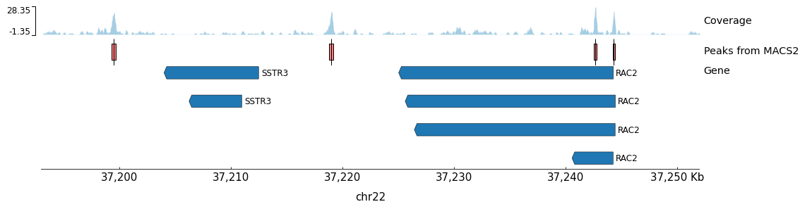
Figure: pyGenomeTracks output showing the chr22:37,193,000-37,252,000 region. The plot displays ATAC-Seq coverage (top track), called peaks (middle track), and gene annotations (bottom track). The peaks correspond to accessible chromatin regions, with the highest peak overlapping with the TSS of the RAC2 gene.

Key Benefits

1. ATAC-Seq Optimized Parameters: The workflow uses ATAC-Seq-specific parameters (shift -100, extsize 200) as recommended by standard tutorials
2. Complete Output Files: Generates all essential outputs including peaks, summits, and bedGraph files for downstream analysis
3. Integrated Visualization: Seamlessly visualizes peaks with coverage and gene annotations
4. Natural Language Interface: Complex peak calling accessible through simple queries
5. Automatic Tool Chaining: Results from peak calling are automatically used for visualization
6. Reproducible Analysis: All tools run in containerized environments with specified versions
7. Human-in-the-Loop Analysis: Users can adjust parameters like extension size, shift, duplicate handling, and visualization regions through natural language

Technical Details

Tool Execution

All tools execute in Docker containers as specified in their CWL definitions:

• macs3: Model-based Analysis of ChIP-Seq (v3.0.3)
• pyGenomeTracks: Genome browser track visualization (v3.9)

macs3 Parameters Explained

Parameter	Value	Description
extsize	200	Extends reads to 200bp fragments
shift	-100	Shifts reads by -100bp (centers on Tn5 cut site)
nomodel	true	Skips fragment size estimation
keepdup	all	Retains all duplicate reads
bdg	true	Outputs bedGraph files for visualization
summits	true	Identifies subpeak summits

Data Flow

1. ATAC-Seq reads (BED format) are processed by macs3
2. macs3 identifies enriched regions (peaks) representing open chromatin
3. Peak summits are identified for precise accessibility positions
4. bedGraph coverage tracks are generated for visualization
5. pyGenomeTracks combines peaks, coverage, and gene annotations into a single plot

Output Files

Step	File	Description
1	*_peaks.narrowPeak	Peak locations (BED6+4 format)
1	*_summits.bed	Peak summit positions
1	*_peaks.xls	Detailed peak statistics
1	*_treat_pileup.bdg	Treatment coverage (bedGraph)
1	*_control_lambda.bdg	Local background estimate
2	*.png	Genome browser visualization

Extending the Workflow

This use case can be extended to:

• Compare peaks between conditions using differential peak analysis
• Annotate peaks with nearby genes using ChIPseeker or HOMER
• Perform motif analysis on peak sequences
• Integrate with RNA-Seq data for multi-omic analysis
• Generate signal heatmaps around transcription start sites
• Identify transcription factor footprints within peaks
• Export peaks to UCSC Genome Browser or IGV

All of these extensions can be implemented by adding additional CWL tools to the MCP server and querying them through natural language.

Reference

Galaxy ATAC-seq tutorial https://galaxyproject.github.io/training-material/topics/epigenetics/tutorials/atac-seq/tutorial.html

MACS3 https://github.com/macs3-project/MACS

pyGenomeTracks https://github.com/deeptools/pyGenomeTracks